Reading: Lookups, Match, and IF Functions

Excel has many powerful functions that can be used to automate calculations and data analysis. In this reading, we will focus on three important functions: VLOOKUP/HLOOKUP, MATCH, and IF/IFS. These functions are essential for working with large datasets and can help you quickly find and manipulate data in Excel.

Before class, you will learn about a few types of IF Statements: IF and IFS. You will also learn about Goal Seek.

VLOOKUP/HLOOKUP Functions

The VLOOKUP and HLOOKUP functions are used to look up values in a table based on a search key. VLOOKUP is used for vertical lookups, while HLOOKUP is used for horizontal lookups. These functions are particularly useful when you have a large dataset and need to find specific information quickly.

The syntax for the VLOOKUP function is as follows:

VLOOKUP(lookup_value, table_array, col_index_num, [range_lookup])

where:

Parameter	Explanation
lookup_value	The value to be found in the first column of the array.
table_array	The table of information in which data is looked up. Use a reference to a range or a range name.
col_index_num	The column number in the table defined by `range` from which the matching value must be returned.
[range_lookup]	A logical value (`TRUE` or `FALSE`) that specifies whether you want VLOOKUP to find an exact match or an approximate match.

The syntax for the HLOOKUP function is similar, but it searches horizontally across rows instead of vertically across columns. For this reading, we will focus on VLOOKUP, but the concepts are similar for HLOOKUP.

Example of VLOOKUP

The following workbook computes the volume and weight of a set of cylinders. The weight is computed from the volume and the unit weight. However, the unit weight depends on the material being used. Unit weights for a set of common materials are shown in a table at the top:

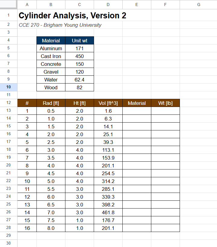
The objective of this example is to determine the appropriate unit weight for each cylinder and calculate the correct weight by multiplying the selected unit weight by the computed volume. We will do this by automatically selecting the correct unit weight from the list using the VLOOKUP function.

For our case, we will use VLOOKUP to select a unit weight value from the table using the user-specified material. The unit weight returned by the function is then multiplied by the volume to compute the cylinder weight as follows:

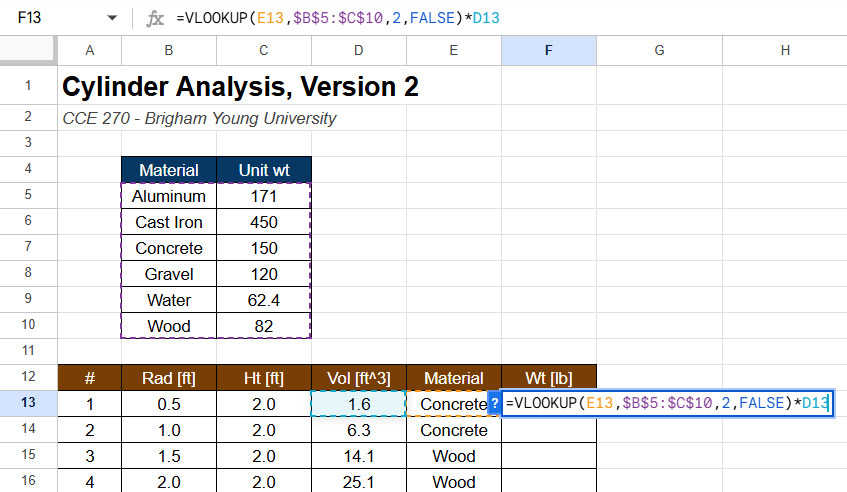
The first argument (E13) to the VLOOKUP function refers to the Material value on the same row and is a relative reference. The second argument ($B$5:$C$10) is an absolute reference to the table use for the lookup. The search_key ("Concrete" in this case) is used to search through the first column in the table to find the row matching the search_key. In this case, the match is found on the third row of the table (cell B7). The third argument (2) tells the VLOOKUP function from which column of the table the return value should be selected. Since the value is 2, we go to the second column of the lookup table on the selected row and find our value (150). This is the value that is returned by the function and multiplied by the volume (1.6) to compute the weight. After copying this formula to the rest of the column, the weight values are all correctly computed as follows:

If the values in the lookup table are edited, all the weights would be automatically updated.

The [range_lookup] Parameter

In the example shown in the previous section, we are doing an exact match on the lookup value in the first column. In some cases we are not looking for an exact match, but we need to find a match from a set of numerical ranges. For example, suppose that we wanted to categorize the cylinder weights using the following guidelines:

Range	Category
wt ≤ 1000	Ultra Light
1000 ≤ wt ≤ 2000	Light
2000 ≤ wt ≤ 10,000	Medium
10,000 ≤ wt ≤ 100,000	Heavy
100,000 ≤ wt	Extra Heavy

We will then add a new table and an extra column as follows:

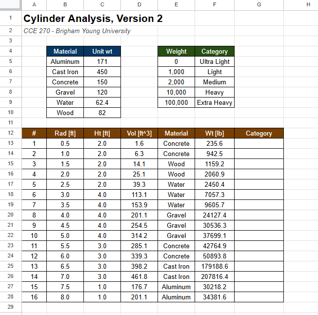
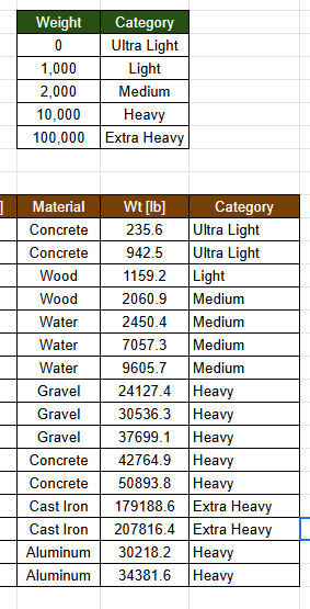
Note that the weight values in the first column of the weight-category table at the top right has been sorted in ascending order. This is critical in order for the lookup to work. Next, we enter a formula using the VLOOKUP function as follows:

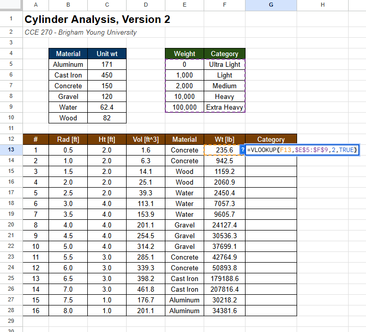
Notice that the last argument (is_sorted) has a value of TRUE. This means that we take the search_key (235.6 in this case) and we look through the first column of the table until we find a row where the value on the row is less than or equal to the search_key and the value on the next row is greater than the search_key. In this case, the match occurs on the first row and so the resulting value from column 2 is "Ultra Light". After copying the formula to the rest of the Category column, the resulting values are as follows:

It is important to note that the is_sorted argument to the VLOOKUP function is optional. If it is omitted, it is assumed to be TRUE by default. A common error with the VLOOKUP function is to omit this argument when the VLOOKUP function is intended to be used as an exact match. This can lead to unintended errors, depending on how the values in the first column are ordered. Therefore, it is strongly recommended to always enter a TRUE or FALSE value for the is_sorted argument every time the VLOOKUP function is used.

Here is an extra resource for further information on VLOOKUP: VLOOKUP

MATCH Function

The MATCH function returns the position of an item in a range of cells. It is often used in conjunction with the VLOOKUP function to find the index of a value in a row or column. The MATCH function can be used to perform exact matches or range lookups, depending on the search type specified.

Let's first look at the syntax of the function.

MATCH(lookup_value, lookup_array, [match_type])

where:

Parameter	Explanation
lookup_value	The value to be found in the range of cells.
lookup_array	The table of information in which data is looked up. Use a reference to a range or a range name.
[match_type]	An optional parameter that directs the function on how to find the `search_key` in the `range`.

The search_type has three different options for an input as shown in the table below. If nothing is input for this parameter, the default value will be 1 which indicates that the values are sorted in ascending order. It will perform a range lookup and return the largest value less than or equal to the search_key. The second value is -1 and works opposite to 1. It indicates that the values are sorted in descending order and perform a range lookup and return the smallest value greater than or equal to the search_key. The last acceptable input is 0. This option directs the function to search for an exact match to the search_key.

Search Type	Explanation
1	Ascending Order (default)
0	Exact Match
-1	Descending Order

The MATCH function when paired with the VLOOKUP function allows you to do a two-dimensional lookup where a value is found from a table containing both rows and columns. For example, consider the following sheet containing a table of temperatures in degree F illustrating a relationship between average monthly temp and elevation in ft for a particular location.

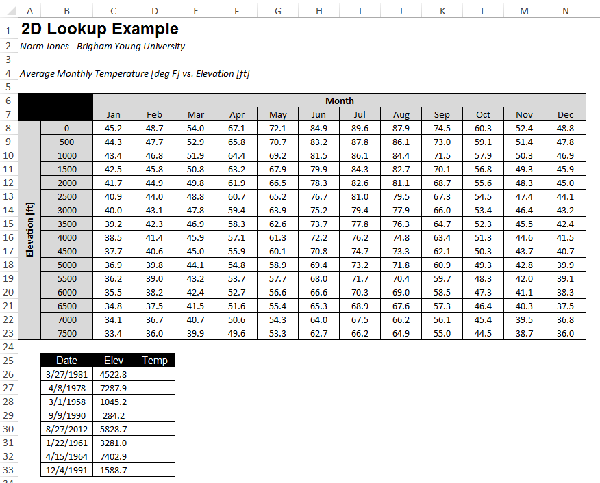
Starting at row 24, another table is listed and the objective is to fill in the Temp column with a formula that looks up the temperature corresponding to the elevation from column C and the month associated with the date provided in column B. This requires a double lookup. We use VLOOKUP to find the row we need based on a range lookup of elevation using the VLOOKUP function. Then, for the third argument to VLOOKUP, we need to determine which column to use based on the month desired. To find the right column based on the month, we first need to find the month label ("Jan", "Feb", etc.) from a date value. This can be accomplished using the TEXT function which takes a date as an argument and returns the month or day value depending on the format specified by the second argument as follows:

TEXT(B28,"MMM")

For the values shown, the function would return "Mar". Then we need to use this text string to automatically find the index of the column corresponding to this month. This can be done with the MATCH function as follows:

MATCH(TEXT(B28,"MMM"),$B$7:$N$7,0)

The first argument to the MATCH function is the lookup value, the second argument is an array (row or column of values) and the third argument indicates the type of match to perform (a value of 0 tells it to find an exact match). The function looks through the array to find the lookup value and returns the index of the item if found. For the arguments shown, the function would return a value of 3. At this point, we are ready to use the VLOOKUP function. We would formulate the function call as follows:

Note that we are using a range lookup on elevation so the last argument to VLOOKUP is TRUE.

Here is an extra resource for further information on Match: MATCH

IF/IFS Functions

IF Statements

IF Statements are a function within Excel that can compare two values and determine if they are true or false. This type of two-outcome expression in programming is known as a boolean.

Syntax

The syntax for an IF statement is as follows:

=IF(logical_expression, value_if_true, value_if_false)

An IF statement has three arguments:

logical_expression: This is what is known as the conditional statement. This function can compare whether a number is greater than (>), less than (<), or if a number or text is equal to (=) in the given condition
value_if_true: This is a placeholder for what will be returned if the given condition is found to be true.
value_if_false: This is a placeholder for what will be returned if the given condition is found to be false.

Example Problem - IF Statement

Let's look at a simple example of an IF statement using strings. Here are a few fictional locations that have different types of material their driveways are made out of. Using an IF statement, we can quickly differentiate for specifically a concrete driveway.

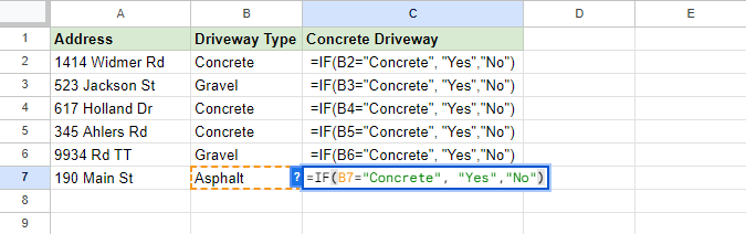
We can write a single statement in cell C2, drag it down, and watch it populate with either a "Yes" or a "No" depending on the conditional statement we gave the function.

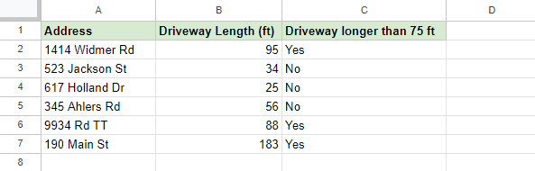
One more example is using a number. Using the length of a driveway, we can find which of the driveways are longer than the given distance of 75 ft.

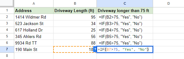
Again, we can see that we can quickly populate the rest of the table by dragging the corner of the cell down.

IFS Statements

IFS Statements are an even more powerful version of an IF statement that can allow for multiple conditional statements to take place within one function. This type of function allows for easy categorization by testing a given number or string against one found in a table.

Syntax

The syntax for an IFS statement is as follows:

=IFS(logical_expression1, value_if_true1, [logical_expression2, value_if_true2], [logical_expression3, ...)

An IFS statement only technically requires two arguments, both of which are nearly the same as the IF statement. However, there can be any number of logical expressions within one IFS statement.

Note: More than one condition can be true so the function will always return the value for the first condition that is found true.

Example Problem - IFS Statement

Using the same premise as the IF statement, we can utilize the table we used before. This time around, we will categorize the different lengths of driveways into three tiers: short, medium, and long.

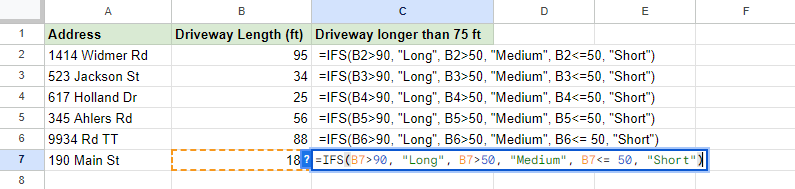
Note: The third condition <=50 includes = so that 50 is included in "less than or equal to 50"

Dragging them down, we can see the final result. Now each driveway is nicely categorized by its length.

Pre-Class Quiz Challenge

First download the starter sheet: (Starter-Workbook)-Pre-Lookups-Match-IF.xlsx
Be sure to make a copy of the sheet and rename it something like “(Your-Name)-Pre-Lookups-Match-IF”.
The workbook contains two sections: the first sheet is for practicing VLOOKUP and MATCH functions, and the second sheet is for practicing IF and IFS functions. Take a minute to review the contents of the LOOKUP-MATCH sheet.

Often times, the VLOOKUP and MATCH functions are hard to understand and use right away. Especially when combining and writing a function inside other functions. To help with this, we will first practice by using each function separately, then combine them together.

In column E, you will use the MATCH function to find the position or index of the type of service listed in column D based on the small table in cells K1:N8. If written correctly, the function will return a number between 2-4, depending on the type of service, listed in column D. We will use this number in the next step. Hint: The entire table in cells K1:N8 is not used for this step.
In column F, you will use the VLOOKUP function to find the cost of the service listed in column B in the table in cells K1:N8. For the index parameter of your VLOOKUP function, you will use the value returned by the MATCH function in column E. If written correctly, the function will return a number, depending on the type of service
In column G, you will multiply the values in columns C and F to get the total cost for each service
In column I, try combining everything you wrote in columns E, F, and G into one formula. The formula should return the total cost for each service based on the service type, quantity, and cost per service

Look below for a solution to see if you did it correctly and for some hints. (Click on the bold words to see the hints)

Solution

For any customer with the Service: "Sidewalk Replacement", Quantity: "10", and Type: "Full", the cost should be $1,890. You can test this by overwriting the formulas that are randomly generated in the "Service" and "Type" columns with these values.

Hint 1: Function Syntax

Column B - Search Key Column C - Multiply the total of your VLOOKUP and Match Function at the end Column D - Search Key for the Index or MATCH Function

Hint 2: N/A Errors

If you are getting a lot of N/As maybe your is_sorted on your Vlookup is not correct or your search type for match is incorrect. Look over the pre-class readings for help

Hint 3: N/A Errors Part 2

Make the is_sorted false and the search type 0

Next, look at the IF-IFS sheet. This sheet is a simple grade book for a class. You will use IF and IFS statements to assign points, pass/fail status, and letter grades to students.

Go to column D ("Points") and use RANDBETWEEN to give points to students randomly. Points should be between 0 and 100. Note that the RANDBETWEEN function will be updated and generate new values each time the sheet is updated. To make the values static, select the entire column, and then copy and paste-special (as values) the results to lock in the values. This overwrites the formula with the values it generated. If you need help, look at the solution below.
In column E, write a simple IF statement in the Pass/Fail column to indicate "Pass" or "Fail" depending on whether they scored over 60/100
In column F, write a complex IF statement in the "Grade" column to assign a letter grade to each student based on their points as follows:

Grading Scale	Letter Grade
90 - 100	A
80 - 89	B
70 - 79	C
60 - 69	D
< 60	F

Look below for a solution to see if you did it correctly and for some hints. (Click on the bold words to see the hints)

RANDBETWEEN Function

=RANDBETWEEN(0,100)

Turning in/Rubric

REMINDER - For this class, you will only turn in the links to your Excel files. You will get a 0 for this assignment if you turn in an Excel file or a link that is not shareable.

On the top right, click the share button --> share --> settings
Click "anyone" at the top, then underneath "More settings", change "can view" to "can edit". Then click apply.
Copy the link, then turn it into Learning Suite in the feedback box for that assignment.

Rubric:

Item	Points Possible
Total	3

The following is not a part of the rubric, but specifies how you can lose points. For example: if you fail to share your link correctly.

Reasons for Points Lost	Amount
Link shared incorrectly	-10%