HW: Graphing and Numerical Solver
Purpose: This assignment tests your ability to use the programs available to you in Excel to solve complex problems. In this assignment, you will proceed to test your knowledge on how to use Goal Seek, the Solver add-in, and organize data through creating various styles of graph.
Getting Started
- First make a copy of the starter sheet here: (Starter-Workbook)-HW-Graphing-and-Solver.xlsx
- Rename it something like "[Your Name]-HW-Graphing-and-Solver"
- Remember to save it in your OneDrive folder that you created in the first assignment.
Part 1 - Asteroid Defense Missile Trajectory
You have just discovered that an asteroid is headed for Earth! You need to determine if the trajectory of an "asteroid-stopping" defense missile will clear the nearby buildings and destroy the asteroid before it impacts with earth. Unfortunately a building is in the way, and you need to know if you can clear it with the current trajectory and land the remains in a safe zone. Your task is to use goal seek to determine the horizontal location of the missile when it reaches the height of the building. Copy and paste your answers into the appropriate cells. If you are right, something magical will happen!
- Navigate to the "Missile Launch" Sheet.
- In cell K21 enter the trajectory equation for the missile in terms of the horizontal distance (X) and the vertical distance (Y). The trajectory equation is given as:
\(y = -(x^2)+ 155 *x\)
- In cell K22 enter a value for the horizontal distance (X) of the missile. This is the value that you will change to find the horizontal location of the missile when it reaches the height of the building. Try entering a very small number first.
- Head to Data > What-If Analysis > Goal Seek. The Goal Seek window will open.
- Set the "Set cell" to K21 (the trajectory equation) and set the "To value" to 50 (the height of the building).
- In the "By changing cell" box, enter K22 (the horizontal distance of the missile).
- Click "OK" to run the Goal Seek. Excel will change the value in K22 to find the horizontal location of the missile when it reaches the height of the building.
- Copy and paste the value of K22 into cell K28 or "1st Location." This is the first horizontal location of the missile when it reaches the height of the building.
- Now, you need to find the second horizontal location of the missile when it reaches the height of the building. To do this, you will need to change the value in K22 to a larger number and run Goal Seek again.
- Copy and paste the value of K22 into cell K29 or "2nd Location." This is the second horizontal location of the missile when it reaches the height of the building.
Congratulations! You have found the horizontal locations of the missile when it reaches the height of the building!
Part 2 - Missile Force Calculation
Now that you've determined the horizontal location of the missile when it reaches the height of the building, you need to find how much force it will take to hit the asteroid and destroy it. The missile is loaded with a payload that will destroy the asteroid on impact, but you need to ensure that the missile has enough force to reach the asteroid.
- Navigate to the Missile & Asteroid Table. This table contains the data for the Missile and the Asteroid. Each table contains the mass and acceleration of the object.
- In cell N31 use the data provided to solve for the force of the missile using the equation: \(F=m*a\)
- In cell Q31 solve for the force of the asteroid using the same equation.
Setting up the Solver
Now that we have all of our data filled out, we are going to find the point where the force of the missile and the asteroid are equal to each other. We are going to do this by changing the acceleration of the missile using Solver. The solver has three basic functions. The "Set Objective" parameter should always be the cell that contains the equation that you want to optimize. You can find a Max, Min, or a specific value. "By Changing Variable Cells" are the cells that you want to change to optimize the objective. "Subject to the Constraints" are the constraints that you want to apply to the optimization.
- Go to Data > Analyze > Solver. The Solver Parameters window will open. Set the objective to cell N31 (the force of the missile) and set the "Value of" to the value in cell Q31 (the force of the asteroid).
- In the "By Changing Variable Cells" box, enter the cell that contains the acceleration of the missile (cell N30).
- Click on "Add" to add a constraint. Set the constraint to be that the acceleration of the missile (cell N30) must be greater than 0. This ensures that the missile has a positive acceleration.
- Click "OK" to close the Add Constraint window.
- Click "Solve" to run the Solver. The Solver will find the optimal acceleration for the missile that will make the force of the missile equal to the force of the asteroid.
Part 3 - Graphing Streamflow Data
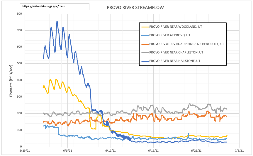
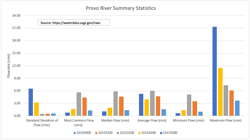
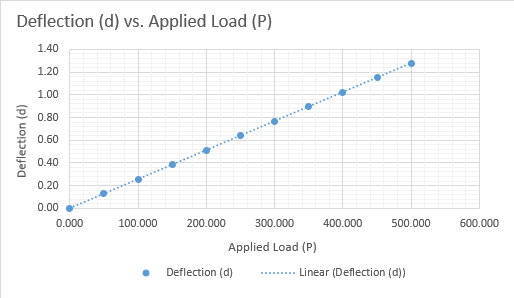
This data comes from USGS Water Data for the Nation and contains streamflow data for the Provo River in Utah. You will be creating three different charts using this data. Each chart should be on its own sheet and should be titled appropriately. The colors of the charts should be changed to something other than the default colors.
- Using the data in the "Streamflow" data sheet recreate this graph. Make sure to change the colors and include a Title, Axis Labels, and a Legend. Put the chart on its own sheet called "Chart 1."
- Using the data in the "Summary Statistics" data sheet recreate this graph. Make sure to change the colors and include a Title, Axis Labels, and a Legend. Put the chart on its own sheet called "Chart 2."
Part 4 - Graphing Load Calculation Data
- Using the data in the "Load Calculations" sheet recreate this graph. Make sure to change the colors and include a Title, Axis Labels, and a Legend. Put the chart on its own sheet called "Chart 3."
Turning in/Rubric
REMINDER - For this class, you will only turn in the links to your Excel files. You will get a 0 for this assignment if you turn in an Excel file or a link that is not shareable.
- On the top right, click the share button --> share --> settings
- Click "anyone" at the top, then underneath "More settings", change "can view" to "can edit". Then click apply.
- Copy the link, then turn it into Learning Suite in the feedback box of the assignment.
Rubric
| Item | Points Possible |
|---|---|
| Part 1: Solved for Vertical Location (Y) | 2 |
| Part 1: Solved for Horizontal Location (X) | 2 |
| Part 1: Found the first location | 2 |
| Part 1: Found the second location | 2 |
| Part 2: Used Force formula for missile | 2 |
| Part 2: Used Force formula for asteroid | 2 |
| Part 2: Added constraint | 1 |
| Part 2: Found equal force by using Solver | 2 |
| Part 3: Chart 1 resembles image | 2 |
| Part 3: Chart 1 is on a separate sheet | 1 |
| Part 3: Chart 2 resembles image | 2 |
| Part 3: Chart 2 is on a separate sheet | 1 |
| Part 4: Chart 3 resembles image | 2 |
| Part 4: Chart 3 is on a separate sheet | 1 |
| Parts 3-4: Charts are all labeled and titled | 6 |
Total |
30 |
The following is not a part of the rubric, but specifies how you can lose points. For example: if you fail to share your link correctly.
| Reasons for Points Lost | Amount |
|---|---|
| Link shared incorrectly | -10% |
| Turned in late (per week) | -10% (up to -50%) |