HW: Numpy
Purpose: Create and use numpy arrays to find the forces in a given truss. You will then use Matplotlib to graph it.
Instructions
-
First, make a copy of the starter sheet here:

-
Rename it something like "(Your_Name)_HW_Numpy.ipynb"
For this assignment, Dr. Doofenshmirtz is partnering with BYU to create a new roof for his building. Instead of a dome, he wants to be fancy and install a triangle roof. He needs you to find the internal forces in each of the segments of his roof truss to ensure it will not collapse. Here is the design of the trusses for his roof:
(image updated from trussanalysis.com)
Where:
- \(L_{AC}\) is the length of segment AC, you will select
- \(θ_A\) and \(θ_C\) are angles at points A and C, respectively that you will select
- P is a load being applied at point B acting downward (denoted with the red arrow)
- Joint A has a pin joint (reaction forces in the x and y direction)
- Joint C has a roller (reaction force only in the y direction)
We want to evaluate a number of truss designs by changing the angles at joints A and C, as well as the length of member AC. The two angles determine how tall the truss is, which is important for Dr. Doofenshmirtz's design. The length of member AC will determine how wide the building is.
For this problem, you will:
1) Select two angles for \(θ_A\) and \(θ_C\) and the length of member \(L_{AC}\).
2) Use numpy to solve for the forces in each segment of the truss.
3) Solve for the lengths of members AB, BC, and AC.
4) Use Matplotlib to graph the truss with the forces in each segment.
We will sum the forces at each joint ( Method of Joints) to create the matrix we will solve using the following equations:
\(\sum F_{A_x} = AB*cos(θ_A) + AC + R_{A_x} = 0\)
\(\sum F_{A_y} = AB*sin(θ_A) + R_{A_y} = 0\)
\(\sum F_{B_x} = -AB*cos(θ_A) + BC*cos(θ_C) = 0\)
\(\sum F_{B_y} = -AB*sin(θ_A) - BC*sin(θ_C) = -P\)
\(\sum F_{C_x} = -BC*cos(θ_C) - AC = 0\)
\(\sum F_{C_y} = BC*sin(θ_C) + R_{C_y} = 0\)
Note
- \(AB\), \(AC\), and \(BC\) are the internal forces in each segment of the truss (these are unknowns we are solving for).
- \(R_{A_x}\) and \(R_{A_y}\) are the reaction forces at joint A (these are unknowns we are solving for).
- \(R_{C_y}\) is the reaction force at joint C (this is an unknown we are solving for).
- \(-P\) is the external load acting downward at joint B (this is a known value we will input).
To solve for these variables, we will arrange the equations so we can create a matrix from the coefficients of the unknowns.
We can then use these equations to solve for our unknown forces: \(AB, AC, BC, R_{A_x}, R_{A_y}\). Typically, this could take a long time when doing it by hand, but can be solved in seconds with some python code and numpy. The way we go about this is by setting up our forces as a system of equations. The equations shown above can be written in matrix form as:
\(\begin{bmatrix} \cos(\theta_A) & 0 & 1 & 1 & 0 & 0 \\ \sin(\theta_A) & 0 & 0 & 0 & 1 & 0 \\ -\cos(\theta_A) & \cos(\theta_C) & 0 & 0 & 0 & 0 \\ -\sin(\theta_A) & -\sin(\theta_C) & 0 & 0 & 0 & 0 \\ 0 & -\cos(\theta_C) & -1 & 0 & 0 & 0 \\ 0 & \sin(\theta_C) & 0 & 0 & 0 & 1 \end{bmatrix} \begin{bmatrix} AB \\ BC \\ AC \\ R_{A_x} \\ R_{A_y} \\ R_{C_y} \end{bmatrix} = \begin{bmatrix} 0 \\ 0 \\ 0 \\ -P \\ 0 \\ 0 \end{bmatrix}\)
In this matrix we know everything in the leftmost matrix and the rightmost matrix. The middle matrix is what we are solving for. For example we input angles \(θ_A\) and \(θ_C\) and the load P. We can solve for \(θ_B\) using the fact that the sum of the angles in a triangle is 180 degrees. Then we know everything we need to know to fill out the matrix.
The \(0\) and \(1\) values in the leftmost matrix come from whether a load in the joint exists for that equation. For example in the first row \([\cos(\theta_A) \quad 0 \quad 1 \quad 1 \quad 0 \quad 0]\) represents the equation for the forces in the x direction at joint A. In this equation, there is a force from member AB in the x direction (hence the \(\cos(\theta_A)\) term), there is no force from member BC in the x direction at joint A (hence the \(0\) term), there is a force from member AC in the x direction (hence the \(1\) term), there is a reaction force at A in the x direction (hence the \(1\) term), and there are no other forces acting on joint A in the x direction (hence the \(0\) terms). The other rows follow the same logic.
The rightmost matrix just contains the load \(-P\) at joint B, and 0's everywhere else since there are no other external loads acting on the truss.
Where the first matrix is our forces matrix (or a matrix of the coefficients), the second matrix is our internal forces which are unknown, this is what we are solving for, and the third matrix is our external forces.
This may seem daunting! But it can be rather simple. Let's jump into it!
We will help by breaking this problem down into 4 parts. This will be confusing, you will need to refer back to the equations and the matrices often to ensure you are putting the right values in the right places. We suggest you write out an outline on paper before you start coding to help organize your thoughts and what you want the code to do. If you can explain step by step what you want the code to do, it will make it much easier to write the code.
Part 1: Solve for the Forces in each segment
We just have to provide the force matrix and the external force matrix to numpy and it will solve for the unknowns in the internal force matrix.
We will write the equations in terms of the angles at A and C, so that we can change the angles and solve the problem again.
We will use functions to solve this problem. This will allow us to call the function multiple times with different inputs. We will create a function that will take in the angles at A and C, and the load at B. This function will return the forces in each segment of the truss. The function will build the force and external load matrices. For this problem, we will hard code the size of these matrices. This is because we know the size of the matrices will not change. The only things that we will allow to change are the angles and the load.
- Import the numpy and Matplotlib library into your notebook.
- In the next code block, create a function that will take in 3 parameters: the angle at joint A (θ_A), the angle at joint C (θ_C), and the load at joint B (P) to find the forces of each member.
Inside the function we now need to do the following:
- Because Numpy works in radians and not degrees, convert the given angles for A and C from degrees to radians. Save those values into variables for the two angles.
Now we need to write the force matrix. This will be a 6x6 matrix. We will use the equations we derived above to create the matrix. The first row will be the coefficients of the first equation, the second row will be the coefficients of the second equation, and so on. The last row will be the external forces acting on the truss. Each row needs to contain coefficients for each of the unknowns. If that unknown is not part of that equation, use a coefficient of 0.
The easiest way to do this is make a matrix for each of the size equations on their own line, then put them together using the square brackets. Here is some example code, you will need to replace the 0's with the actual number or equation. Some of them will still be 0's.
forces = np.array([
    [0, 0, 0, 0, 0, 0],  # forces in the x direction at A
    [0, 0, 0, 0, 0, 0],  # forces in the y direction at A
    [0, 0, 0, 0, 0, 0],  # forces in the x direction at B
    [0, 0, 0, 0, 0, 0],  # forces in the y direction at B
    [0, 0, 0, 0, 0, 0],  # forces in the x direction at C
    [0, 0, 0, 0, 0, 0]   # forces in the y direction at C
])
The order of both the unknowns and the external forces is important. They can be in any order, but each of the three arrays has to use the same order.
- Create the force coefficient matrix. Make each row in our matrix represent a given equation. Start by creating the equation for joint A in the x direction. Note you can make each of these rows a separate numpy array with a variable name, then put them together in the end. This will make it easier to read and debug.
The array should be in the same order as the other arrays, if you follow the examples, \(A_x\) should be the first row, \(A_y\) should be the second row, etc. Save this array as a variable such as combined_forces.
- Now, create a new array for the external forces acting on the truss using the given solution matrix in the introduction. Save this as a variable such as loads. Make sure it is in the same order.
- We can now solve this! Using your force coefficient and external loads arrays, solve the system of equations. Have your force coefficient array be the first input and your external forces the second. Refer back to your in-class work back with what numpy function to use with solving systems of equations. Save this as a variable such as solutions. This will give you the values for \(AB\), \(AC\), \(BC\), \(R_{AY}\), \(R_{AX}\), and \(R_{CY}\).
- You are given a dictionary to store these values for each member/location. It looks like
total_forces = {"AB":0, "BC":0, "AC":0, "R_AX":0, "R_AY":0, "R_CY":0}, with the 0's replaced by the actual forces. This dictionary has already been created for you. - With your solved values, you will now update the dictionary total_forces. You will update the values of the dictionary with the values you got from your system of equations. For example, my dictionary would say something like "AB": 3000, "R_AY": -200 when updated. The dictionary will be used later.
- Write a loop that will print the values of the dictionary with the solutions you got from your system of equations. For example, my print statement would say something like "AB = 3000 lbs", "R_AY = -200 lbs, etc." when displayed.
- Return this dictionary from your function.
Part 2: Find Coordinates of each point
Now that you have all the forces, Dr. Doofenshmirtz needs to know how high his roof is going to be. This will involve solving for the x and y coordinates of joints A, B, and C. We are going to use trigonometry to solve for the coordinates of each joint and the trig functions in numpy to do the calculations.
We will create a function that will accept \(θ_A\), \(θ_C\) and \(L_{AC}\) as inputs, then calculate the coordinates of each of the corners. We will use the sum of the angles to get \(θ_B\). We will divide the truss into two right triangles and use the law of sines to get the base and hypotenuse. Using that information, we can solve for the x and y coordinates of each joint.
- Create a new function that will take in 3 parameters: \(θ_A\), \(θ_C\) and \(L_{AC}\) as inputs. This function will solve for the X and y values of each joint. (We will say that A is the origin with coordinates [0,0])
- Since we are given angle A (\(θ_A\)) and angle C (\(θ_C\)), solve for angle B (\(θ_B\)). Hint: the sum of the angles in a triangle is 180 degrees.
- Convert angles A, B, and C from degrees to radians (since this is what Numpy does its calculations in)
- Time to bring back your geometry skills, now that you know all of your angles and one side length you can use the law of sines to solve for the other lengths. Save each length of the truss in their own variables.
Here is the law of sines for reference where a, b, and c are the lengths of each side opposite their respective angles A, B, and C:
(image from CalcWorkshop)
So for example to solve for length AB you would use the equation:
If you set the following variables:
length_AC = length of the truss member from A to C
angle_B   = angle at joint B in radians
angle_C   = angle at joint C in radians
length_AB = length of the truss member from A to B
Here is some example python code to solve the equation for length AB. You will need to replace the variable names with your own variable names as needed.:
length_AB = (length_AC / np.sin(angle_B)) * np.sin(angle_C)
Hint
- It may be helpful to setup a separate function to solve for the lengths using the law of sines to avoid repeating code. Your main function can then call this helper function three times to get the lengths of AB, BC, and AC.
- you may want to have several simpler functions your main function calls to help break down the problem into smaller pieces.
- It will also probably be helpful to outline this on paper before you start coding
- Print the length of AB, BC, and AC with the respective units. For example, my print statement would say something like "Length of AB: 3 ft", "Length of BC: 4 ft", "Length of AC: 6 ft" when displayed.
- Now that you have all of your lengths, you can solve for the x and y coordinates of each joint. To do this, you will use the following equations:
- For joint A, the x and y coordinates are both 0 (we are saying that A is the origin). Save both the x and y coordinates as a singular variable such as joint_A that is a list of two values.
- For joint B, the x coordinate is the length of AB times the cosine of angle A. The y coordinate is the length of AB times the sine of angle A. Save this as a variable such as joint_B.
- For joint C, the x coordinate is the length of AC. The y coordinate 0 since it is the same level as A. Save this as a variable such as joint_C.
- Create a dictionary to store these values. The keys will be the joint names (A, B, C) and the values will be the x and y coordinates of each joint. For example, your dictionary might look like
"A": (0, 0), "B": (3, 4), "C": (6, 0)when displayed. - Return this dictionary if you used a function to create it.
Note
- It will probably be helpful to outline this on paper before you start coding
- This doesn't need a lot of detail, just the steps you need to take to solve the problem.
- Each of the steps are relatively simple, but there are a lot of them. Breaking them down will help you avoid mistakes.
- If you start coding before organizing your thoughts, you may find yourself going back and redoing a lot of work.
Part 3: Graph the Truss
Now that we have solved for the forces and the coordinates of each joint, we can graph the truss. The objective is to graph each segment of the truss in either blue or red. Blue will represent a tension (positive) force, and red will represent a compressive (negative) force. You will then label each joint with the letter of the joint (A, B, C). We will use the dictionary to loop through the different members, determine if the force is negative or positive for a color, then plot a line from the beginning coordinates to the end coordinates. For example for member \(AC\) we would plot a line from coordinates of A to the coordinates of C.
This code will be given to you as a preview for the next topic.
Part 4: Call Functions
- Create inputs statements that prompt the user for the angle at joint A (degrees), the angle at joint C (degrees), the load at joint B (upwards is positive and downwards is negative), and the length of AC (feet). Save these as variables.
- Call the function that solves for the forces in each segment. Pass in the angle at joint A, the angle at joint C, and the load at joint B as parameters. Save the output as a variable such as forces.
- Call the function that solves for the coordinates of each joint. Pass in the angle at joint A, the angle at joint C, and the length of AC as parameters. Save the output as a variable such as coordinates.
- Call the function that graphs the truss. Pass in the forces and coordinate functions as parameters.
- Run each code block and test it with the following values:
- Test 1:
- Angle at joint A: 60 degrees
- Angle at joint C: 30 degrees
- Load at joint B: -2000 lbs
- Length of AC: 10 ft
- Expected output:

- Test 2:
- Angle at joint A: 35 degrees
- Angle at joint C: 55 degrees
- Load at joint B: -3000 lbs
- Length of AC: 25 ft
- Expected output:

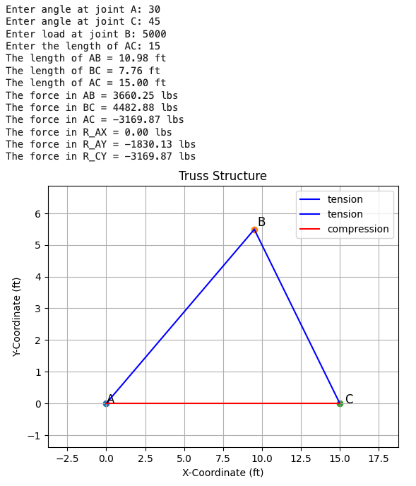
- Test 3:
- Angle at joint A: 30 degrees
- Angle at joint C: 45 degrees
- Load at joint B: 5000 lbs
- Length of AC: 15 ft
- Expected output:
Turning in/Rubric
REMINDER - For this class, you will only turn in the links to your colab notebooks. You will get a 0 for this assignment if you turn in a python file or a link that is not correct, wrong assignment, or does not give editor permission.
Rubric:
| Items | Amount |
|---|---|
| Part 1: Correctly constructs the force equilibrium equations and loads in matrix form based on the given matrix. | 4 |
| Part 1: solution is added to the total_forces dictionary and dictionary is returned and printed | 3 |
| Part 2: Side lengths AB, BC, and AC are found and printed | 3 |
| Part 2: Coordinates for A, B, and C are added to the coordinates dictionary, returned, and printed | 3 |
| Part 3: If statements are used to create the correct labeling and coloring based on positive (tension, blue) and negative (compression, red) force values | 3 |
| Part 3: Graph contains: title, x/y labels, legend for tension/compression, and labels for each point | 3 |
| Part 4: Values for forces, lengths, and coordinates match given test scenarios | 4 |
| Part 4: Graph matches given test scenarios | 4 |
| Comments are added to explain code | 3 |
Total |
30 |
The following is not a part of the rubric, but specifies how you can lose points. For example: if you do not explain your code when using AI to help you create it or fail to share your link correctly.
| Reasons for Points Lost | Amount |
|---|---|
| Link shared incorrectly | -10% |
| Turned in late (per week) | -10% (up to -50%) |
| No comments explaining where AI is used and what its provided code does | -50% |