Reading: Pivot Tables, Goal Seek, and Data Validation
Data Validation
Data validation is a feature in Excel that allows you to control the type of data entered into a cell. This can be useful to ensure that the data entered into a cell is appropriate for the context of how it will be used. For example, you may have a formula that only works with positive values. You can use data validation to ensure that the cell(s) used as input to the formula only accepts positive values. This is different from filtering data as data validation controls the data that can be entered into a cell while filtering data changes the range of data you see. Data validation can help prevent errors in your data and make it easier to work with.
Let's go over how to add data validation to your data in Excel:
- Select the range of cells you want to add data validation to.
- Click on Data | Data Validation.
- In the data validation criteria box, you can set up the criteria for the data that can be entered into the cells. For example, you can choose to allow only numbers, text, dates, or a list of items.
- You can also choose the output of the data validation you want to apply to the cells. For example, you can choose to show a warning message if the data entered does not meet the criteria or to reject the data altogether.
- Once you have set up the criteria and output options, click on Save to apply the data validation to the selected range of cells.
Note
You can also add multiple data validation rules to the same range of cells. For example, you can set up a rule that allows only numbers and another rule that allows only dates.
Dropdown
This is useful when you want to limit the data that can be entered into a cell to a specific list of items. For example, you can create a drop-down list of options for a cell that allows the user to select from a list of items. To do this, follow the same steps as above and select List. You can then enter the items you want to include in the drop-down list. In the example below, the data validation is set up to allow only the values in the drop-down list to be entered into the cells.
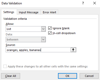
If you're wanting to create a drop-down list from a range of cells, you can select the range of cells that contain the items you want to include in the drop-down list. This is useful when you have a long list of items that you want to include in the drop-down list.
Dates
This is useful when you want to limit the data that can be entered into a cell to a specific date range. For example, you can create a data validation that only allows dates between 6/1/2021 and 6/30/2021 to be entered into the cells. To do this, follow the same steps as above and select the criteria that best fit the date range you want your data to have. In the example below, the data validation is set up to allow only dates between 6/1/2021 and 6/30/2021 to be entered into the cells.
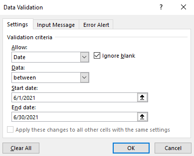
There are many other options for data validation. Here is an extra resource for further examples of Data Validation: Data Validation
Pivot Tables
Pivot Tables are used to summarize and analyze large sets of data in more meaningful ways. They can be used to narrow down data sets and see relationships between data points among other things. Pivot tables allow us to summarize multiple columns and rows of data at a time.
For example, here is a data set showing sales data. If you would like to follow along, you can use this data set: reg_sales_data.xlsx
The data set shows the sales data for a set of regional sales managers. The data set includes region, the product, the name of the sales rep, the number of units sold, and the total sales. Now suppose we want to create a summary of the units sold and the total sales in each region, organized by sales rep. We could manually extract that information from the table, or we could use some combination of COUNTIF and SUMIF to accomplish this. Or we could find that information in a few clicks using a pivot table. The following steps show how to create a pivot table in Excel.
Creating the Pivot Table
- First, we select the data set. In this case, we select the cells in the range A1:F31.
- Next, we select the Insert|Pivot Table option from the menu. This will bring up the following dialog box:

We can either choose to put the pivot table in a new sheet or in the existing sheet. In this case, we will put the pivot table in an existing sheet named "summary." We will click the "Ok" button. This will create a pivot table in the existing "summary" sheet. The empty pivot table will look like this:

Editing the Pivot Table
Now we need to decide what data we want to summarize in the pivot table. We can do this using the Pivot table editor on the right. The editor will look like this:

Now we can start adding data to the pivot table. Adding data to the pivot table is done by dragging and dropping the desired data into the appropriate sections in the editor. The sections are Filters, Rows, Columns, and Values.
- Go to the editor and click and drag the Region category into the Rows section.
- Click on the Sales Rep option and drag it to the Rows section.
At this point you should see a list of regions and the sales reps for each region in the pivot table. This data set is a little odd in that the same sales rep is listed in multiple regions, so apparently the sales reps are not limited to work in a single region. Now we need to add the data that we want to summarize.
- Click and drag the Units Sold option to the Values section. If you click on Sum of Units Sold | Value Field Settings you'll notice that the "Summarize Values By" option is set to "Sum." This means that the pivot table will show the sum of the units sold for each sales rep in each region. You can also summarize by min, max, average, count, and other options. Let's keep the default of "Sum" for now.
- Click and drag the Total Sales option to the Values section. Once again, the default is to summarize by sum.
At this point, the pivot table should look like this:

Now we can see the total units sold and total sales for each sales rep in each region. As you can see, it only takes a few clicks to create a pivot table that summarizes a large data set in a meaningful way. Pivot tables are fun!
Additional Readings
Below are some links to additional readings on pivot tables.
- Introduction Excel PivotTable
- Create a PivotTable to Analyze Worksheet Data
- Pivot Tables in Excel (bonus functions of pivot tables)
Goal Seek
In many Excel computations, we encounter equations that are too complex or impractical to solve directly. Instead, we often rely on an iterative, trial-and-error approach—adjusting input values until the formula produces the desired result. Goal Seek is a function in Excel that automates this process. It is a powerful tool that utilizes an algorithm that plugs in different calculations to find a solution for an unknown variable using a known end-goal value. One example of this is often found in sales when determining how many units need to be sold to break even or meet a certain quota.
Using Goal Seek
To use Goal Seek, head to Data | What-If Analysis | Goal Seek. This will open the Goal Seek dialog box, where you can enter your desired values and the cells you want to change.
Goal Seek has three basic components:
- Set Cell
- To Value
- By Changing Cell
Example Problem
Let's use the example of a contractor wanting to find what he would have to charge to make a profit of $1250 by building his friend a 12' x 12' deck. Given the cost of materials ($6000) and the $22/hr of pay for each employee, we can calculate the project cost. Using Goal Seek, we can allow the computer to do the rest of the work for us.
First, click the Set Cell grid icon on the Goal Seek tab, then select the cell you want to set.
Hint: This cell should almost always be the cell that contains your formula.

Then, set the To Value to whatever value you are trying to find. In our case, this number would be 1250.
Finally, select the cell that would need to change to evaluate the final part of the question. In this instance, this would be cell B9.
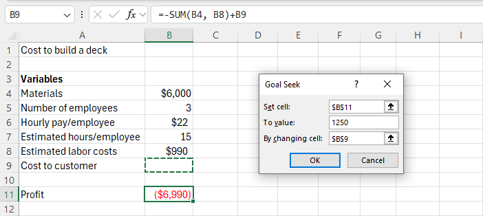
When all three inputs are filled on the Goal Seek tab, the Solve button will light up blue. If you press the button, the computer should start jumping between values trying to find the solution to what gets a profit of $1250.
In this example, our solution is $8240.000057, or $8240!
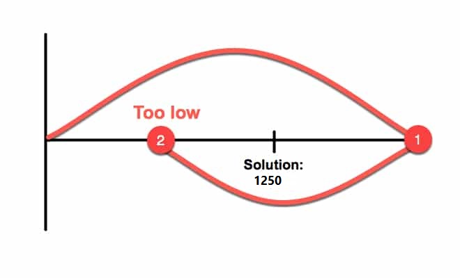
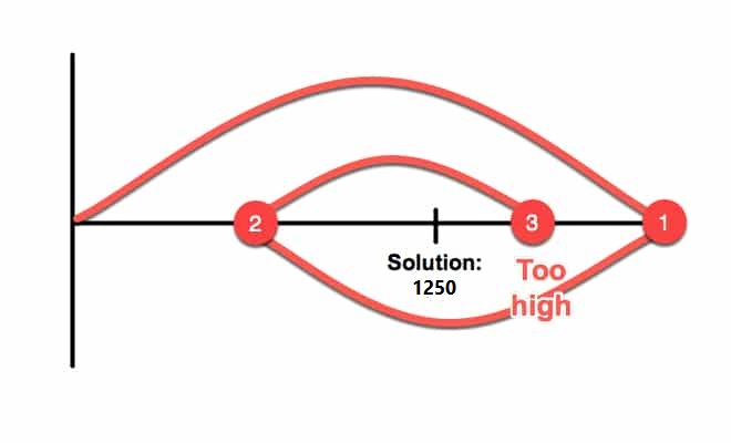
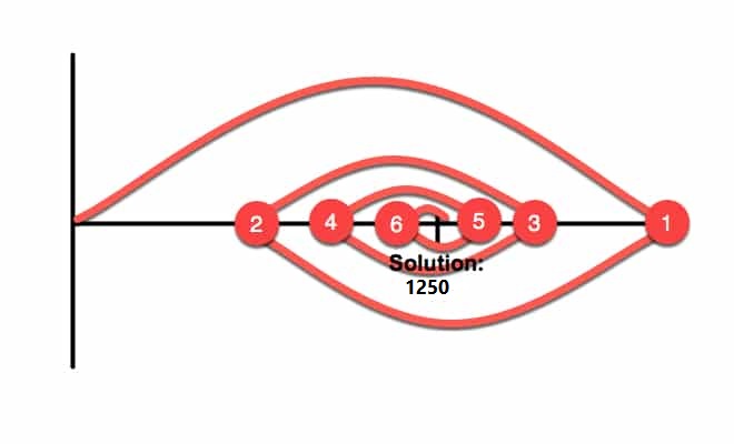
How does this work?
Each attempt by the computer tries to get closer and closer by guessing a number.
Attempt 1
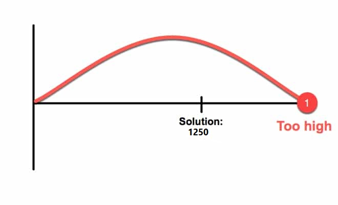
Attempt 2
Attempt 3
Attempt 4 and onwards
Pre-Class Quiz Challenge
Here is a link for the pre-class starter sheet: (Starter-Workbook)-Pre-Pivot-GoalSeek-DataV.xlsx
Make sure to rename it something like “(Your-Name)-Pre-Pivot-GoalSeek-DataV.” Note that this is an expanded version of the regional sales data set that we used in the pivot table example above.
Part 1: Data Validation
Navigate to the "Dogshow" sheet, and use the Data Validation tool (found under the Data tab) to limit:
- The breed of dogs (C6:C23) to the list provided.
- The judges' scores (D6:F23) to whole numbers 0 - 10.
- The winners (C28:C30) to the names of entered dogs.
Fill in the red chart to check your data validation (randomly select breeds and individual judge scores). Enter a Sum function for the total scores. Then enter the names and scores of the 1st, 2nd, and 3rd place winners.
Part 2: Pivot Table
- Select the entire table on the "Reg_sales_data" sheet and create a pivot table in the existing "PivotTable" sheet.
- Drag and drop Sales Rep and Product into the rows section in that order. Then add the Units Sold (Sum) and Total Sales (Sum) into the value category. This will summarize the total units sold and total sales for each sales rep for each product.
Part 3: Goal Seek
Navigate to the "Fishing" sheet.
You are out fly-fishing, when a huge fish jumps high out of the water to eat your fly. You just happen to know the parabolic equation that all trout jumps follow which is:
\(y = -(x-2)^2 + 5\)
You want to figure out how far it jumped.
- Use goal seek to determine the two \(x\) values that make \(y = 0.\)
- Copy your answers into C28 and C29.
- As an extra curiosity, you want to figure out how high the fish jumped. Input the average of the two \(x\) values in cell E28 to find the max \(y\) value.
Turning in/Rubric
REMINDER - For this class, you will only turn in the links to your Excel files. You will get a 0 for this assignment if you turn in an Excel file or a link that is not shareable.
- On the top right, click the share button --> share --> settings
- Click "anyone" at the top, then underneath "More settings", change "can view" to "can edit". Then click apply.
- Copy the link, then turn it into Learning Suite in the feedback box for that assignment.
Rubric:
| Item | Points Possible |
|---|---|
Total |
3 |
The following is not a part of the rubric, but specifies how you can lose points. For example: if you fail to share your link correctly.
| Reasons for Points Lost | Amount |
|---|---|
| Link shared incorrectly | -10% |