In-Class Exercise: NumPy
The following exercises will have you create and manipulate arrays. For this exercise, open the in-class workbook, make a copy, and follow the instructions.
You can find the In Class Exercise here:

Instructions
- Open the in-class workbook using the link above.
- Rename it something like "(Your_Name)_Class_Numpy.ipynb"
- Follow the instructions in the notebook to complete the exercise.
Vectorized Operations in NumPy
NumPy is a powerful library for numerical computing in Python. One of the key features of NumPy is its ability to perform vectorized operations on arrays. Vectorized operations are operations that are applied to each element of an array. For example, if you have two arrays a and b, you can add them together element-wise using the + operator:
import numpy as np

a = np.array([1, 2, 3])
b = np.array([4, 5, 6])

c = a + b
print(c)  # Output: [5 7 9]
Speed of vectorized operations
NumPy vectorization is much faster than using a for loop to iterate over the elements of an array. This is because NumPy uses optimized C code to perform the operations, whereas a for loop in Python is interpreted and slower. Here is an example of how much faster NumPy vectorization is compared to a for loop. We create two numpy arrays with 1 million members each and add them together using both a for loop and NumPy vectorization. We then use the %timeit command to measure the time it takes to run each operation. :
import numpy as np

# function to add two arrays using loops
def plusarray(x1, x2):
  x3 = np.zeros(len(x1))
  for i in range(len(x1)):
    x3[i] = x1[i] + x2[i]
  return x3


# two arrays with 1 million members
x4 = np.random.rand(1000000)
x5 = np.random.rand(1000000)

print('Numpy vectorization')
%timeit x4 + x5

print('Function using loops')
%timeit plusarray(x4, x5)
Which results in the following output:
Numpy vectorization
1.5 ms ± 169 µs per loop (mean ± std. dev. of 7 runs, 1000 loops each)

Function using loops
590 ms ± 151 ms per loop (mean ± std. dev. of 7 runs, 1 loop each)
The %timeit command is a magic command in Colab notebooks that measures the time it takes to run a piece of code. The output shows that the NumPy vectorization is about 400 times faster than the function using loops. This is because NumPy uses optimized C code to perform the operations, whereas a for loop in Python is interpreted and slower.
Last part in In-Class Exercise Explanation
Truss Analysis with NumPy
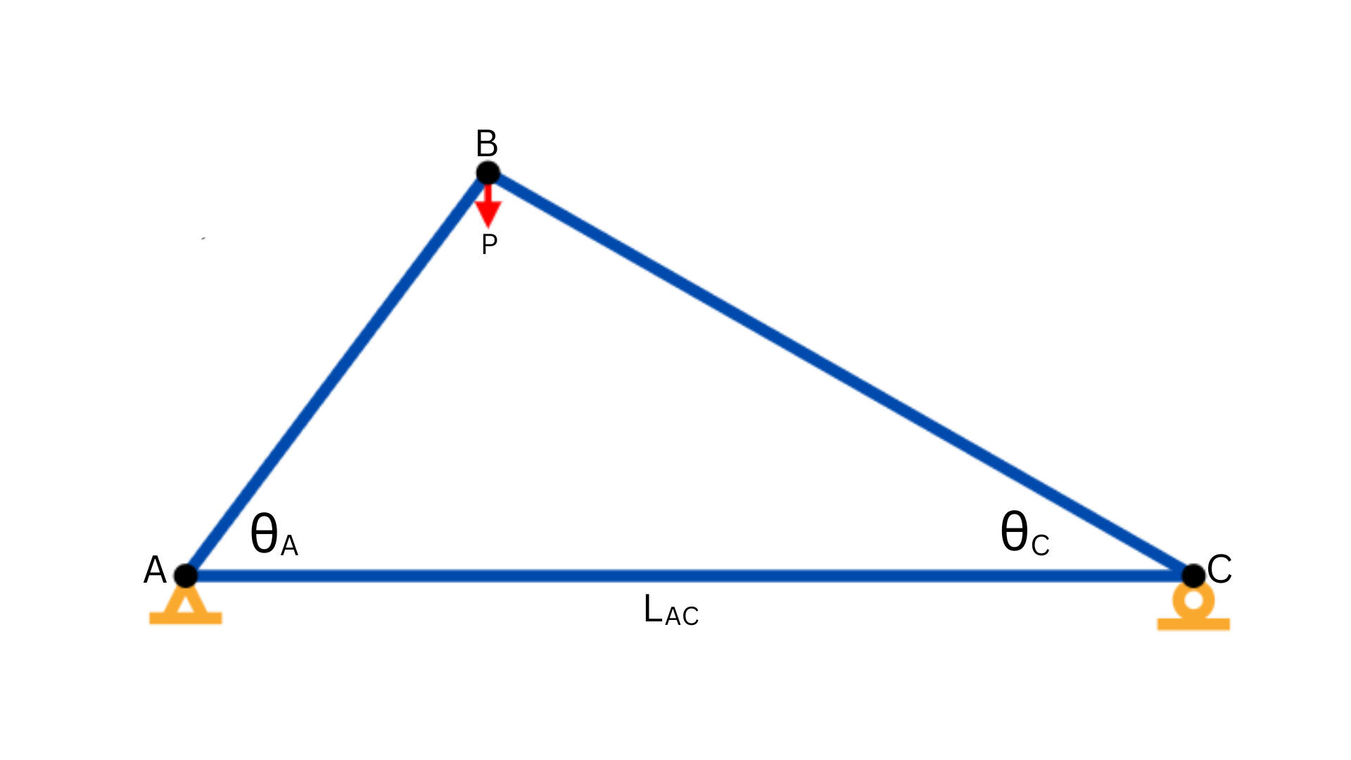
We will use a truss as an example of solving simultaneous equations. A truss is a structure made up of members that are connected at their ends. The members are usually made of steel or wood and are used to support loads. The truss in the image above is a simple truss with three members and three joints. The members are labeled AB, BC, and AC. The joints are labeled A, B, and C. The loads are applied at joint B and joint C.
To create mathematical equations to solve a truss, we need to express the forces in terms of the given angles and loads. Here are the equations derived from the matrices:
Equilibrium Equations
-
Sum of Forces in the x-direction for each joint have to equal 0:
\(F_{A_x}: \cos(\theta_A) \cdot F_{AB} + 1 \cdot F_{AC} + 1 \cdot R_{A_x} = 0\)
\(F_{B_x}: -\cos(\theta_A) \cdot F_{AB} + \cos(\theta_C) \cdot F_{BC} = 0\)
\(F_{C_x}: -\cos(\theta_C) \cdot F_{BC} - 1 \cdot F_{AC} = 0\)
-
Sum of Forces in the y-direction for each joint have to equal 0:
\(F_{A_y}: \sin(\theta_A) \cdot F_{AB} + 1 \cdot R_{A_y} = 0\)
\(F_{B_y}: -\sin(\theta_A) \cdot F_{AB} - \sin(\theta_C) \cdot F_{BC} = -P\)
\(F_{C_y}: \sin(\theta_C) \cdot F_{BC} + 1 \cdot R_{C_y} = 0\)
Note: Even though P is shown in the diagram as acting in the negative y-direction, we treat it as a positive value in the derivation. It has a minus sign after moving it from the left-hand side to the right-hand side. With this solution, for a force P acting downward, we would enter a negative value for P. If P were acting upward, we would enter a positive value for P.
We can now "line up" the equations in a matrix form to solve for the unknowns.
The matrix form of the equations is:
You may recognize this as a system of linear equations, which are typically referenced as \(Ax = b\), where \(A\) is the matrix of coefficients, \(x\) is the vector of unknowns, and \(b\) is the vector of knowns. The big matrix on the left is a set of coefficients we have derived based on statics and geometry. The vector on the right (mostly zeros) represents the known loads on the truss, and the vector in the middle corresponds to the unknown x vector and it represents the forces in the members and the reactions at the supports.
For reference, here are our coefficients and loads in table format. Note: If you compare this table to the equations above, you will notice that we have changed the order of the equations so that the two A equations are first, followed by the two B equations, and finally the two C equations. Also, we switched the order of 2nd and 3rd columns.
| AB | BC | AC | RAx | RAy | RCy | |
|---|---|---|---|---|---|---|
| FAx | cos(θA) | 0 | 1 | 1 | 0 | 0 |
| FAy | sin(θA) | 0 | 0 | 0 | 1 | 0 |
| FBx | -cos(θA) | cos(θC) | 0 | 0 | 0 | 0 |
| FBy | -sin(θA) | -sin(θC) | 0 | 0 | 0 | 0 |
| FCx | 0 | -cos(θC) | -1 | 0 | 0 | 0 |
| FCy | 0 | sin(θC) | 0 | 0 | 0 | 1 |
| Loads | |
|---|---|
| FAx | 0 |
| FAy | 0 |
| FBx | 0 |
| FBy | -P |
| FCx | 0 |
| FCy | 0 |
As you may recall, it is possible to solve a system of linear equations. This can be rather cumbersome, but fortunately, there is a simple way to do it in NumPy using the np.linalg.solve() function. Once you have formulated the A matrix and the b vector, you can solve for the unknowns using the following code:
import numpy as np

x = np.linalg.solve(A, b)
For the in-class, and homework exercises, you will be given the equations and the knowns. You will need to use NumPy to solve for the unknowns.
Turning in/Rubric
REMINDER - For this class, you will only turn in the links to your colab notebooks. You will get a 0 for this assignment if you turn in a python file or a link that is not correct, wrong assignment, or does not give editor permission.
Rubric:
| Item | Points Possible |
|---|---|
Total |
5 |
The following is not a part of the rubric, but specifies how you can lose points. For example: if you fail to share your link correctly.
| Reasons for Points Lost | Amount |
|---|---|
| Link shared incorrectly | -10% |
| Turned in late (per week) | -10% (up to -50%) |